5. Multilayer Perceptron

5.1. Sigmoid function

BP algorithm is mainly due to the emergence of Sigmoid function, instead of the previous threshold function to construct neurons.

The Sigmoid function is a monotonically increasing nonlinear function. When the threshold value is large enough, the threshold function can be approximated.

../../_images/mlp_1.jpg

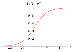
The Sigmoid function is usually written in the following form:

\[f(x) = \frac{1}{1 + e^{-x}}\]

The value range is \((-1,1)\), which can be used instead of the neuron step function:

\[f(x) = \frac{1}{1 + e^{- \sum_{i=1}^{n} w_i x_i-w_0}}\]

Due to the complexity of the network structure, the Sigmoid function is used as the transfer function of the neuron. This is the basic idea of multilayer perceptron backpropagation algorithm.

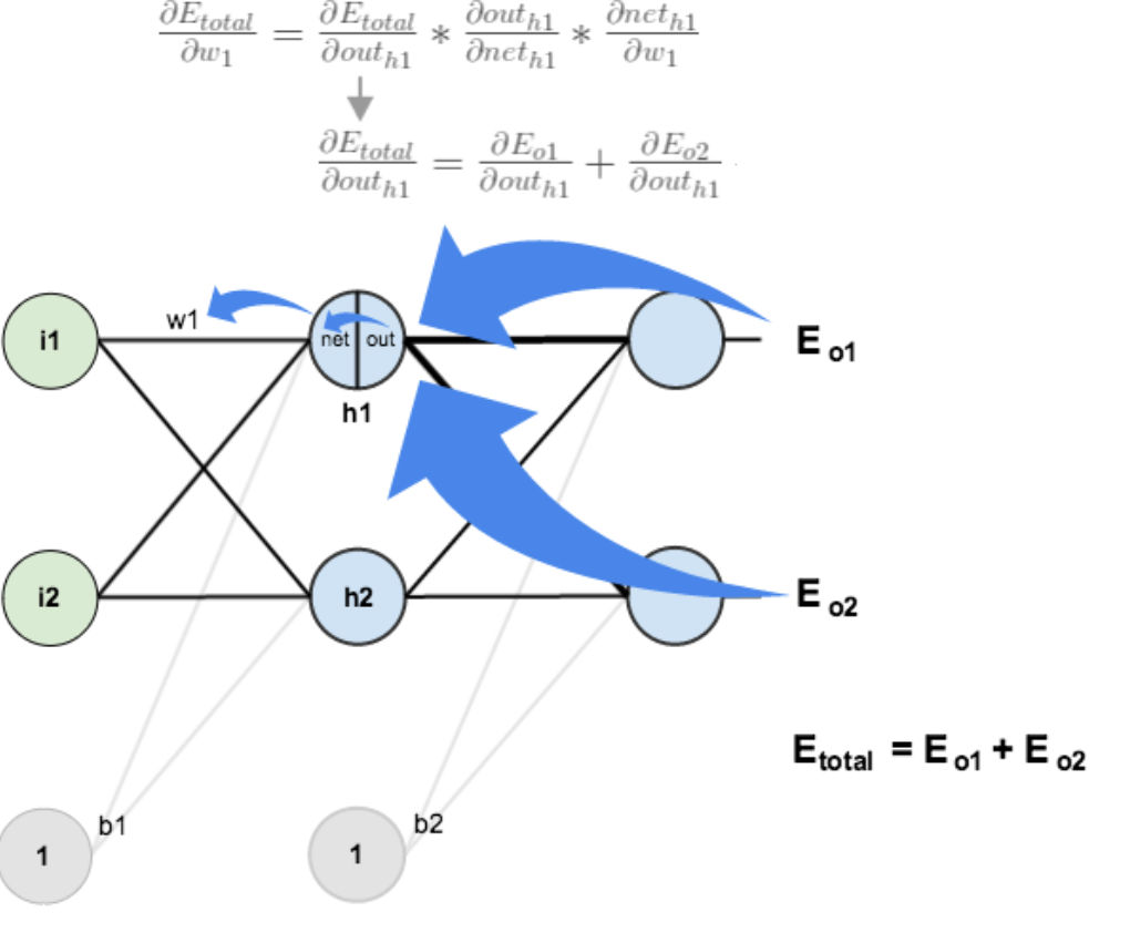
5.2. Back Propagation

Back Propagation (BP) algorithm is the optimization of the network through the iterative weights makes the actual mapping relationship between input and output and the desired mapping, descent algorithm by adjusting the layer weights for the objective function to minimize the gradient. The sum of the squared error between the predicted output and the expected output of the network on one or all training samples:

\[\begin{split}& J(w) = \frac{1}{2} \sum_{j=1}^{s} (t_j - s_j)^2 = \frac{1}{2} \mid t - a \mid ^ 2 \\ & J_{total}(w) = \frac{1}{2} \sum_{i=1}^{N} \mid t_i - a_i \mid ^ 2\end{split}\]

The error of each unit is calculated by layer by layer error of output layer:

\[\begin{split}\bigtriangledown w_j^k & = - \eta \frac{\partial J}{\partial J w_j^k} \\ & = - \eta \frac{\partial J}{\partial n_j^k}\frac{\partial n_j^k}{\partial Jw_j^k} \\ & = -\eta \frac{\partial J}{\partial n_j^k} a^{k-1} \\ & = - \eta \delta_j^k a^{k-1}\end{split}\]

Back Propagation Net (BPN) is a kind of multilayer network which is trained by weight of nonlinear differentiable function. BP network is mainly used for:

  1. function approximation and prediction analysis: using the input vector and the corresponding output vector to train a network to approximate a function or to predict the unknown information;
  2. pattern recognition: using a specific output vector to associate it with the input vector;
  3. classification: the input vector is defined in the appropriate manner;
  4. data compression: reduce the output vector dimension to facilitate transmission and storage.

For example, a three tier BP structure is as follows:

../../_images/mlp_2.png

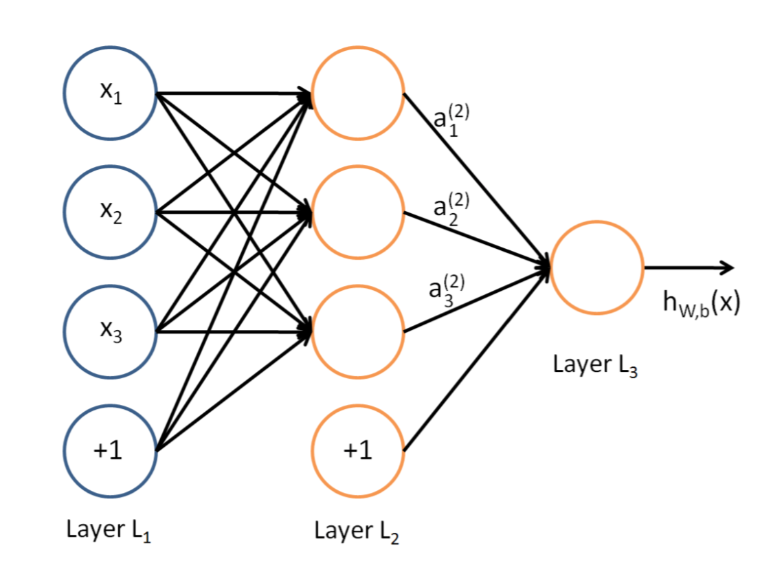
It consists of three layers: input layer, hidden layer and output layer. The unit of each layer is connected with all the units of the adjacent layer, and there is no connection between the units in the same layer. When a pair of learning samples are provided to the network, the activation value of the neuron is transmitted from the input layer to the output layer through the intermediate layers, and the input response of the network is obtained by the neurons in the output layer. Next, according to the direction of reducing the output of the target and the direction of the actual error, the weights of each link are modified from the output layer to the input layer.

5.3. Example

Suppose you have such a network layer:

  • The first layer is the input layer, two neurons containing \(i_1, i_2, b_1\) and intercept;
  • The second layer is the hidden layer, including two neurons \(h_1, h_2\) and intercept b2;
  • The third layer is the output of \(o_1, o_2\) and \(w_i\) are each line superscript connection weights between layers, we default to the activation function sigmoid function.

Now give them the initial value, as shown below:
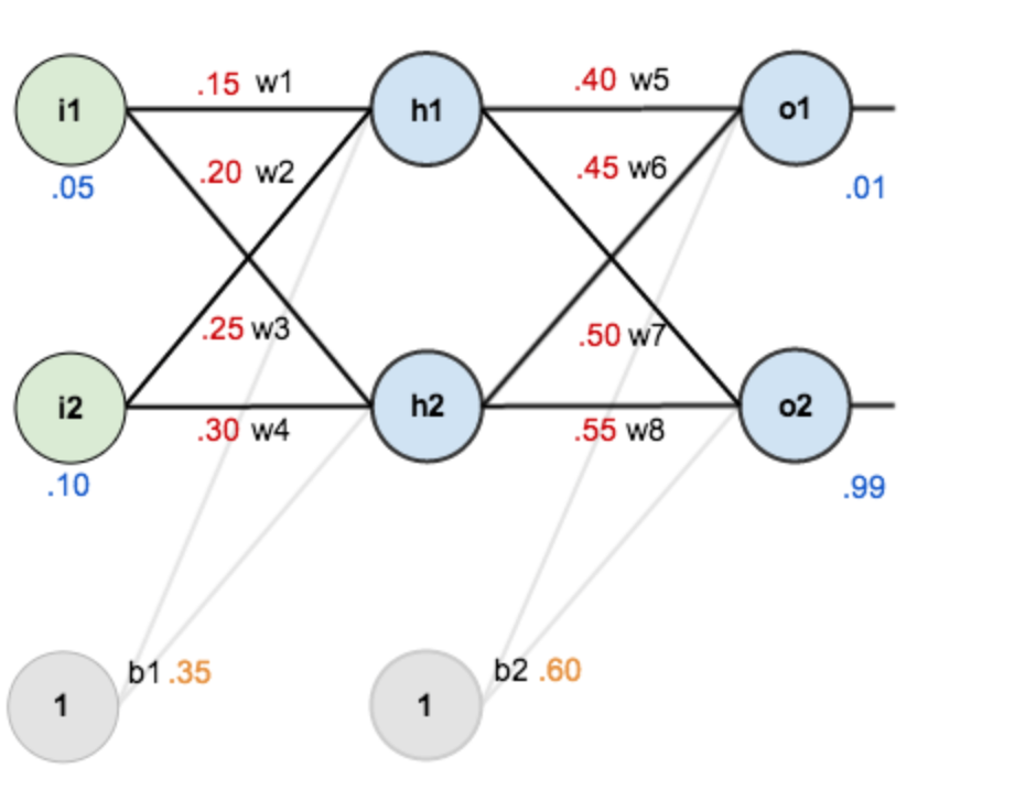
../../_images/mlp_3.png

Among them,

  • Input data: \(i_1=0.05, i_2=0.10\);
  • Output data: \(o_1=0.01, o_2=0.99\);
  • Initial weight: \(w_1=0.15, w_2=0.20, w_3=0.25, w_4=0.30, w_5=0.40, w_6=0.45, w_7=0.50, w_8=0.88\);

Objective: to give input data \(i_1, i_2\) (0.05 and 0.10), so that the output is as close as possible to the original output \(o_1, o_2\) (0.01 and 0.99).

5.3.1. Step 1: Forward Propagation

5.3.1.1. Input layer to Hidden layer

Calculate the input weighted sum of neurons \(h_1\):

\[\begin{split}& net_{h1} = w_1 * i_1 + w_2 * i_2 + b_i * 1 \\ & net_{h1} = 0.15 * 0.05 + 0.2 * 0.1 + 0.35 * 1 = 0.3775\end{split}\]

\(o_1\), the output of neuron \(h_1\): (Activation function sigmoid is required here):

\[out_{h1} = \frac{1}{1 + e^{-net_{h1}}} = \frac{1}{1+e^{-0.3775}} = 0.593269992\]

Similarly, \(o_2\), the output of neuron \(h_2\) can be calculated:

\[out_{h2} = 0.596884378\]

5.3.1.2. Hidden layer to Output layer

The values of \(o_1\) and \(o_2\) in the output layer are calculated:

\[\begin{split}& net_{o1} = w_5 * out_{h1} + w_6 * out_{h2} + b_2 * 1 \\ & net_{o1} = 0.4 * 0.593269992 + 0.45 * 0.596884378 + 0.6 * 1 = 1.105905967 \\ & out_{o1} = \frac{1}{1+e^{-net_{o1}}} = \frac{1}{1+e^{-1.105905967}} = 0.75136507 \\ & out_{o2} = 0.772928465\end{split}\]

This propagation process is finished, we get the output value of \([0.75136079, 0.772928465]\), and the actual value of \([0.01, 0.99]\) far from now, we for the error back-propagation, update the weights, to calculate the output.

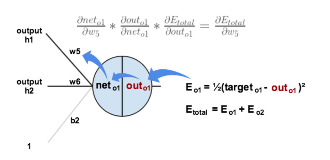
5.3.2. Step 2: Back Propagation

5.3.2.1. Calculate the total error

Total error (square error):

\[E_{total} = \sum \frac{1}{2}(target - output) ^ 2\]

For example, the target output for \(o_1\) is 0.01 but the neural network output 0.75136507, therefore its error is:

\[E_{o1} = \frac{1}{2}(target_{o1} - out_{o1}) ^ 2 = \frac{1}{2} (0.01 - 0.75136507)^2 = 0.274811083\]

Repeating this process for \(o_2\) (remembering that the target is 0.99) we get:

\[E_{o2} = 0.023560026\]

The total error for the neural network is the sum of these errors:

\[E_{total} = E_{o1} + E_{o2} = 0.274811083 + 0.023560026 = 0.298371109\]

5.3.2.2. Hidden layer to Hidden layer weights update

Take the weight parameter \(w_5\) as an example, if we want to know how much impact the \(w_5\) has on the overall error, we can use the global error to obtain the partial derivative of \(w_5\): (chain rule)

\[\frac{\partial E_{total}}{\partial w_5} = \frac{\partial E_{total}}{\partial out_{o1}} * \frac{\partial out_{o1}}{\partial net_{o1}} * \frac{\partial net_{o1}}{\partial w_5}\]

The following figure can be more intuitive to see how the error is spread back:

../../_images/mlp_4.png

Now we were calculated for each value:

  • Calculate \(\frac{\partial E_{total}}{\partial out_{o1}}\).
\[\begin{split}& E_{total} = \frac{1}{2}(target_{o1} - out_{o1}) ^ 2 + \frac{1}{2}(target_{o2} - out_{o2}) ^ 2 \\ & \frac{\partial E_{total}}{\partial out_{o1}} = 2 * \frac{1}{2}(target_{o1} - out_{o1})^{2-1} * -1 + 0 \\ & \frac{\partial E_{total}}{\partial out_{o1}} = -(target_{o1} - out_{o1}) = -(0.01 - 0.75136507) = 0.74136507\end{split}\]
  • Calculate \(\frac{\partial out_{o1}}{\partial net_{o1}}\):
\[\begin{split}& out_{o1} = \frac{1}{1+e^{-net_{o1}}} \\ & \frac{\partial out_{o1}}{\partial net_{o1}} = out_{o1} (1-out_{o1}) = 0.75136507(1-0.75136507) = 0.186815602\end{split}\]
  • Calculate \(\frac{\partial net_{o1}}{\partial w_5}\):
\[\begin{split}& net_{o1} = w_5 * out_{h1} + w_6 * out_{h2} + b_2 * 1 \\ & \frac{\partial net_{o1}}{\partial w_5} = 1 * out_{h1} * w_5^{(1-1)} + 0 + 0 = out_{h1} = 0.593269992\end{split}\]
  • Putting it all together:
\[\begin{split}& \frac{\partial E_{total}}{\partial w_5} = \frac{\partial E_{total}}{\partial out_{o1}} * \frac{\partial out_{o1}}{\partial net_{o1}} * \frac{\partial net_{o1}}{\partial w_5} \\ & \frac{\partial E_{total}}{\partial w_5} = 0.74136507 * 0.186815602 * 0.59326992 = 0.082167041\end{split}\]

In this way, we calculate the overall error \(E_{total}\) to the \(w_5\) partial guide. Look at the above formula, we found:

\[\frac{\partial E_{total}}{\partial w_5} = -(target_{o1} - out_{o1}) * out_{o1}(1-out_{o1}) * out_{h1}\]

In order to express convenience, \(\delta_{o1}\) is used to express the error of output layer:

\[\begin{split}& \delta_{o1} = \frac{\partial E_{total}}{\partial out_{o1}} * \frac{\partial out_{o1}}{\partial net_{o1}} = \frac{\partial E_{total}}{\partial net_{o1}} \\ & \delta_{o1} = - (target_{o1} - out_{o1}) * out_{o1} (1-out_{o1})\end{split}\]

Therefore, the overall error \(E_{total}\) can be written as a partial derivative formula for \(w_5\):

\[\frac{\partial E_{total}}{\partial w_5} = \delta_{o1} out_{h1}\]

If the output layer error meter is negative, it can also be written:

\[\frac{\partial E_{total}}{\partial w_5} = - \delta_{o1} out_{h1}\]

Finally, we update the value of \(w_5\):

\[w_5^+ = w_5 - \eta * \frac{\partial E_{total}}{\partial w_5} = 0.4 - 0.5*0.082167041 = 0.35891648\]

Among them, \(\eta\) is the learning rate, here we take 0.5. Similarly, update \(w_6\), \(w_7\), \(w_8\):

\[\begin{split}& w_6^+ = 0.408666186 \\ & w_7^+ = 0.511301270 \\ & w_8^+ = 0.561370121\end{split}\]

5.3.2.3. Hidden layer to Input layer weights update

In fact, with the method above said almost, but there is a need to change, calculate the total error of the above \(w_5\) guide, from \(out_{o1}\) —-> \(net_{o1}\) —-> \(w_5\), but in the hidden layer between the weight update, \(out_{h1}\) —-> \(net_{h1}\) —-> \(w_1\) and \(out_{h1}\) will accept \(E_{o1}\) and \(E_{o2}\) error of two places to two, so this place will be calculated.

../../_images/mlp_5.png
  • Calculate \(\frac{\partial E_{total}}{\partial out_{h1}}\):
\[\frac{\partial E_{total}}{\partial out_{h1}} = \frac{\partial E_{o1}}{\partial out_{h1}} + \frac{\partial E_{o2}}{\partial out_{h1}}\]
  • Calculate \(\frac{\partial E_{o1}}{\partial out_{h1}}\):
\[\begin{split}& \frac{\partial E_{o1}}{\partial out_{h1}} = \frac{\partial E_{o1}}{\partial net_{o1}} * \frac{\partial net_{o1}}{\partial out_{h1}} \\ & \frac{\partial E_{o1}}{\partial net_{o1}} = \frac{\partial E_{o1}}{\partial out_{o1}} * \frac{\partial net_{o1}}{\partial out_{h1}} = 0.74136507 * 0.186815602 = 0.138498562 \\ & net_{o1} = w_5 * out_{h1} + w_6 * out_{h2} + b_2 * 1 \\ & \frac{\partial net_{o1}}{\partial out_{h1}} = w_5 = 0.40 \\ & \frac{\partial E_{o1}}{\partial out_{h1}} =\frac{\partial E_{o1}}{\partial net_{o1}} * \frac{\partial net_{o1}}{\partial out_{h1}} = 0.138498562 * 0.40 = 0.055399425\end{split}\]
  • Similarly, calculate \(\frac{\partial E_{o2}}{\partial out_{h1}} = -.019049119\):
  • Therefore,
\[\frac{\partial E_{total}}{\partial out_{h1}} = \frac{\partial E_{o1}}{\partial out_{h1}} + \frac{\partial E_{o2}}{\partial out_{h1}} = 0.055399425 + -.019049119 + 0.036350306\]
  • Then, calculate \(\frac{\partial out_{h1}}{\partial net_{h1}}\):
\[\begin{split}& out_{h1} = \frac{1}{1+e^{-net_{h1}}} \\ & \frac{\partial out_{h1}}{\partial net_{h1}} = out_{h1} (1-out_{h1}) = 0.241300709\end{split}\]
  • Calculate \(\frac{\partial net_{h1}}{\partial w_{h1}}\):
\[\begin{split}& net_{h1} = w_1 * i_1 + w_2 * i_2 + b_1 * 1 \\ & \frac{\partial net_{h1}}{\partial w_{h1}} = i_1 = 0.05\end{split}\]

Putting it all together:

\[\frac{\partial E_{total}}{\partial w_1} = \frac{\partial E_{total}}{\partial out_{h1}} * \frac{\partial out_{h1}}{\partial net_{h1}} * \frac{\partial net_{h1}}{\partial w_1} = 0.036350306 * 0.241300709 * 0.05 = 0.000438568\]

In order to simplify the formula, \(\sigma_{h1}\) is used to represent the error of the hidden layer unit \(h_1\):

\[\begin{split}& \frac{\partial E_{total}}{\partial w_1}= (\sum_{o}\frac{\partial E_{total}}{\partial out_o} * \frac{\partial out_o}{\partial net_o} * \frac{\partial net_o}{\partial out_{h1}}) * \frac{\partial out_{h1}}{\partial net_{h1}} * \frac{\partial net_{h1}}{\partial w_1} \\ & \frac{\partial E_{total}}{\partial w_1}= (\sum_o \delta_o * w_{ho}) * out_{h1} (1- out_{h1}) * i_1 \\ & \frac{\partial E_{total}}{\partial w_1}= = \delta_{h1} i_1\end{split}\]

We can now update \(w_1\):

\[w_1^+ = w_1 - \eta * \frac{\partial E_{total}}{\partial w_1} = 0.15 - 0.5 * 0.000438568 = 0.149780716\]

Repeating this for \(w_2\), \(w_3\), and \(w_4\):

\[\begin{split}& w_2^+ = 0.19956143 \\ & w_3^+ = 0.24975114 \\ & w_4^+ = 0.29950229\end{split}\]

Finally, we’ve updated all of our weights! When we fed forward the 0.05 and 0.1 inputs originally, the error on the network was 0.298371109. After this first round of back propagation, the total error is now down to 0.291027924. It might not seem like much, but after repeating this process 10,000 times, for example, the error plummets to 0.000035085. At this point, when we feed forward 0.05 and 0.1, the two outputs neurons generate 0.015912196 (vs 0.01 target) and 0.984065734 (vs 0.99 target).

5.4. Code

First, import necessary packages:

import random
import math

Define network:

class NeuralNetwork:
    LEARNING_RATE = 0.5

    def __init__(self, num_inputs, num_hidden, num_outputs,
                 hidden_layer_weights=None,
                 hidden_layer_bias=None,
                 output_layer_weights=None,
                 output_layer_bias=None):
        self.num_inputs = num_inputs

        self.hidden_layer = NeuronLayer(num_hidden, hidden_layer_bias)
        self.output_layer = NeuronLayer(num_outputs, output_layer_bias)

        self.init_weights_from_inputs_to_hidden_layer_neurons(hidden_layer_weights)
        self.init_weights_from_hidden_layer_neurons_to_output_layer_neurons(output_layer_weights)

    def init_weights_from_inputs_to_hidden_layer_neurons(self, hidden_layer_weights):
        weight_num = 0
        for h in range(len(self.hidden_layer.neurons)):
            for i in range(self.num_inputs):
                if not hidden_layer_weights:
                    self.hidden_layer.neurons[h].weights.append(random.random())
                else:
                    self.hidden_layer.neurons[h].weights.append(hidden_layer_weights[weight_num])
                weight_num += 1

    def init_weights_from_hidden_layer_neurons_to_output_layer_neurons(self, output_layer_weights):
        weight_num = 0
        for o in range(len(self.output_layer.neurons)):
            for h in range(len(self.hidden_layer.neurons)):
                if not output_layer_weights:
                    self.output_layer.neurons[o].weights.append(random.random())
                else:
                    self.output_layer.neurons[o].weights.append(output_layer_weights[weight_num])
                weight_num += 1

    def inspect(self):
        print('------')
        print('* Inputs: {}'.format(self.num_inputs))
        print('------')
        print('Hidden Layer')
        self.hidden_layer.inspect()
        print('------')
        print('* Output Layer')
        self.output_layer.inspect()
        print('------')

    def feed_forward(self, inputs):
        hidden_layer_outputs = self.hidden_layer.feed_forward(inputs)
        return self.output_layer.feed_forward(hidden_layer_outputs)

    # Uses online learning, ie updating the weights after each training case
    def train(self, training_inputs, training_outputs):
        self.feed_forward(training_inputs)

        # 1. Output neuron deltas
        pd_errors_wrt_output_neuron_total_net_input = [0] * len(self.output_layer.neurons)
        for o in range(len(self.output_layer.neurons)):
            # ∂E/∂zⱼ
            pd_errors_wrt_output_neuron_total_net_input[o] = self.output_layer.neurons[
                o].calculate_pd_error_wrt_total_net_input(training_outputs[o])

        # 2. Hidden neuron deltas
        pd_errors_wrt_hidden_neuron_total_net_input = [0] * len(self.hidden_layer.neurons)
        for h in range(len(self.hidden_layer.neurons)):

            # We need to calculate the derivative of the error with respect to the output of each hidden layer neuron
            # dE/dyⱼ = Σ ∂E/∂zⱼ * ∂z/∂yⱼ = Σ ∂E/∂zⱼ * wᵢⱼ
            d_error_wrt_hidden_neuron_output = 0
            for o in range(len(self.output_layer.neurons)):
                d_error_wrt_hidden_neuron_output += pd_errors_wrt_output_neuron_total_net_input[o] * \
                                                    self.output_layer.neurons[o].weights[h]

            # ∂E/∂zⱼ = dE/dyⱼ * ∂zⱼ/∂
            pd_errors_wrt_hidden_neuron_total_net_input[h] = d_error_wrt_hidden_neuron_output * \
                                                             self.hidden_layer.neurons[
                                                                 h].calculate_pd_total_net_input_wrt_input()

        # 3. Update output neuron weights
        for o in range(len(self.output_layer.neurons)):
            for w_ho in range(len(self.output_layer.neurons[o].weights)):
                # ∂Eⱼ/∂wᵢⱼ = ∂E/∂zⱼ * ∂zⱼ/∂wᵢⱼ
                pd_error_wrt_weight = pd_errors_wrt_output_neuron_total_net_input[o] * self.output_layer.neurons[
                    o].calculate_pd_total_net_input_wrt_weight(w_ho)

                # Δw = α * ∂Eⱼ/∂wᵢ
                self.output_layer.neurons[o].weights[w_ho] -= self.LEARNING_RATE * pd_error_wrt_weight

        # 4. Update hidden neuron weights
        for h in range(len(self.hidden_layer.neurons)):
            for w_ih in range(len(self.hidden_layer.neurons[h].weights)):
                # ∂Eⱼ/∂wᵢ = ∂E/∂zⱼ * ∂zⱼ/∂wᵢ
                pd_error_wrt_weight = pd_errors_wrt_hidden_neuron_total_net_input[h] * self.hidden_layer.neurons[
                    h].calculate_pd_total_net_input_wrt_weight(w_ih)

                # Δw = α * ∂Eⱼ/∂wᵢ
                self.hidden_layer.neurons[h].weights[w_ih] -= self.LEARNING_RATE * pd_error_wrt_weight

    def calculate_total_error(self, training_sets):
        total_error = 0
        for t in range(len(training_sets)):
            training_inputs, training_outputs = training_sets[t]
            self.feed_forward(training_inputs)
            for o in range(len(training_outputs)):
                total_error += self.output_layer.neurons[o].calculate_error(training_outputs[o])
        return total_error

Define layer:


class NeuronLayer:
    def __init__(self, num_neurons, bias):

        # Every neuron in a layer shares the same bias
        self.bias = bias if bias else random.random()

        self.neurons = []
        for i in range(num_neurons):
            self.neurons.append(Neuron(self.bias))

    def inspect(self):
        print('Neurons:', len(self.neurons))
        for n in range(len(self.neurons)):
            print(' Neuron', n)
            for w in range(len(self.neurons[n].weights)):
                print('  Weight:', self.neurons[n].weights[w])
            print('  Bias:', self.bias)

    def feed_forward(self, inputs):
        outputs = []
        for neuron in self.neurons:
            outputs.append(neuron.calculate_output(inputs))
        return outputs

    def get_outputs(self):
        outputs = []
        for neuron in self.neurons:
            outputs.append(neuron.output)
        return outputs


Define neuron: .. literalinclude:: mlp_bp.py

start-after:neuron-start
end-before:neuron-end

Put all together, and run example:


nn = NeuralNetwork(2, 2, 2,
                   hidden_layer_weights=[0.15, 0.2, 0.25, 0.3],
                   hidden_layer_bias=0.35,
                   output_layer_weights=[0.4, 0.45, 0.5, 0.55],
                   output_layer_bias=0.6)
for i in range(10000):
    nn.train([0.05, 0.1], [0.01, 0.99])
    print(i, round(nn.calculate_total_error([[[0.05, 0.1], [0.01, 0.99]]]), 9))

    # XOR example:

    # training_sets = [
    #     [[0, 0], [0]],
    #     [[0, 1], [1]],
    #     [[1, 0], [1]],
    #     [[1, 1], [0]]
    # ]

    # nn = NeuralNetwork(len(training_sets[0][0]), 5, len(training_sets[0][1]))
    # for i in range(10000):
    #     training_inputs, training_outputs = random.choice(training_sets)
    #     nn.train(training_inputs, training_outputs)
    #     print(i, nn.calculate_total_error(training_sets))

Please Enjoy!

[1]Wikipedia article on Backpropagation. http://en.wikipedia.org/wiki/Backpropagation#Finding_the_derivative_of_the_error
[2]Neural Networks for Machine Learning course on Coursera by Geoffrey Hinton. https://class.coursera.org/neuralnets-2012-001/lecture/39
[3]The Back Propagation Algorithm. https://www4.rgu.ac.uk/files/chapter3%20-%20bp.pdf