1. Activation
1.1. What is activation function?
In computational networks, the activation function of a node defines the output of that node given an input or set of inputs. In biologically inspired neural networks, the activation function is usually an abstraction representing the rate of action potential firing in the cell.

1.2. Why need activation function?
Neural networks compose several functions in layers: the output of a previous layer is the input to the next layer. If you compose linear functions, these functions are all linear. So the result of stacking several linear functions together is a linear function. Using a nonlinear function makes the map from the input to the output nonlinear.
For example, a ReLU function’s output is either 0 or positive. If the unit is 0, it is effectively “off,” so the inputs to the unit are not propagated forward from that function. If the unit is on, the input data is reflected in subsequent layers through that unit. ReLU itself is not linear, and neither is the composition of several layers of several ReLU functions. So the mapping from inputs to classification outcomes is not linear either.
Without activation function many layers would be equivalent to a single layer, as each layer (without an activation function) can be represented by a matrix and a product of many matrices is still a matrix:
1.3. Commonly used activation functions
Every activation function (or non-linearity) takes a single number and performs a certain fixed mathematical operation on it. There are several activation functions you may encounter in practice:
1.3.1. Sigmoid
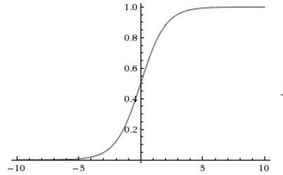
Sigmoid non-linearity squashes real numbers to range between \([0,1]\).
The sigmoid non-linearity has the mathematical form \(σ(x)=1/(1 + e ^ {−x})\) and is shown in the image above. It takes a real-valued number and “squashes” it into range between 0 and 1. In particular, large negative numbers become 0 and large positive numbers become 1. The sigmoid function has seen frequent use historically since it has a nice interpretation as the firing rate of a neuron: from not firing at all (0) to fully-saturated firing at an assumed maximum frequency (1). In practice, the sigmoid non-linearity has recently fallen out of favor and it is rarely ever used. It has two major drawbacks:
- Sigmoids saturate and kill gradients. A very undesirable property of the sigmoid neuron is that when the neuron’s activation saturates at either tail of 0 or 1, the gradient at these regions is almost zero. Recall that during backpropagation, this (local) gradient will be multiplied to the gradient of this gate’s output for the whole objective. Therefore, if the local gradient is very small, it will effectively “kill” the gradient and almost no signal will flow through the neuron to its weights and recursively to its data. Additionally, one must pay extra caution when initializing the weights of sigmoid neurons to prevent saturation. For example, if the initial weights are too large then most neurons would become saturated and the network will barely learn.
- Sigmoid outputs are not zero-centered. This is undesirable since neurons in later layers of processing in a Neural Network (more on this soon) would be receiving data that is not zero-centered. This has implications on the dynamics during gradient descent, because if the data coming into a neuron is always positive (e.g. \(x > 0\) elementwise in \(f = w ^ T x + b\))), then the gradient on the weights \(w\) will during backpropagation become either all be positive, or all negative (depending on the gradient of the whole expression \(f\)). This could introduce undesirable zig-zagging dynamics in the gradient updates for the weights. However, notice that once these gradients are added up across a batch of data the final update for the weights can have variable signs, somewhat mitigating this issue. Therefore, this is an inconvenience but it has less severe consequences compared to the saturated activation problem above.
1.3.2. Tangent
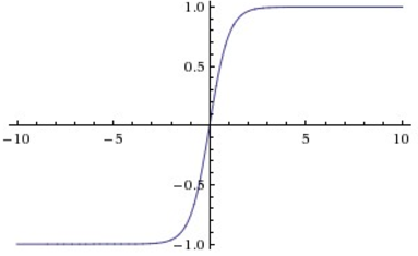
The tanh non-linearity squashes real numbers to range between \([-1,1]\).
The tanh non-linearity is shown on the image above. It squashes a real-valued number to the range \([-1, 1]\). Like the sigmoid neuron, its activations saturate, but unlike the sigmoid neuron its output is zero-centered. Therefore, in practice the tanh non-linearity is always preferred to the sigmoid nonlinearity. Also note that the tanh neuron is simply a scaled sigmoid neuron, in particular the following holds:
1.3.3. ReLU
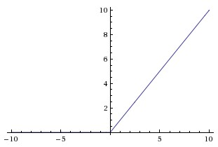
Rectified Linear Unit (ReLU) activation function, which is zero when \(x < 0\) and then linear with slope \(1\) when \(x > 0\).
The Rectified Linear Unit has become very popular in the last few years. It computes the function
In other words, the activation is simply thresholded at zero (see image above). There are several pros and cons to using the ReLUs:
- (+) It was found to greatly accelerate (e.g. a factor of 6 in Krizhevsky et al [1].) the convergence of stochastic gradient descent compared to the sigmoid/tanh functions. It is argued that this is due to its linear, non-saturating form.
- (+) Compared to tanh/sigmoid neurons that involve expensive operations (exponentials, etc.), the ReLU can be implemented by simply thresholding a matrix of activations at zero.
- (-) Unfortunately, ReLU units can be fragile during training and can “die”. For example, a large gradient flowing through a ReLU neuron could cause the weights to update in such a way that the neuron will never activate on any datapoint again. If this happens, then the gradient flowing through the unit will forever be zero from that point on. That is, the ReLU units can irreversibly die during training since they can get knocked off the data manifold. For example, you may find that as much as 40% of your network can be “dead” (i.e. neurons that never activate across the entire training dataset) if the learning rate is set too high. With a proper setting of the learning rate this is less frequently an issue.
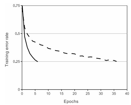
A plot from Krizhevsky et al. [1] paper indicating the 6x improvement in convergence with the ReLU unit compared to the tanh unit.
1.3.4. Leaky ReLU
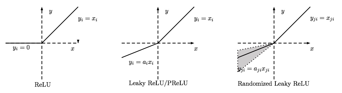
Leaky ReLUs are one attempt to fix the “dying ReLU” problem. Instead of the function being zero when \(x < 0\), a leaky ReLU will instead have a small negative slope (of \(0.01\), or so). That is, the function computes
where \(α\) is a small constant. Some people report success with this form of activation function, but the results are not always consistent. The slope in the negative region can also be made into a parameter of each neuron, as seen in PReLU neurons, introduced in Delving Deep into Rectifiers, by Kaiming He et al., 2015 [2]. However, the consistency of the benefit across tasks is presently unclear.
1.3.5. Maxout
Other types of units have been proposed that do not have the functional form
where a non-linearity is applied on the dot product between the weights and the data. One relatively popular choice is the Maxout neuron (introduced recently by Goodfellow et al [3].) that generalizes the ReLU and its leaky version. The Maxout neuron computes the function
Notice that both ReLU and Leaky ReLU are a special case of this form (for example, for ReLU we have \(w1,b1=0\)). The Maxout neuron therefore enjoys all the benefits of a ReLU unit (linear regime of operation, no saturation) and does not have its drawbacks (dying ReLU). However, unlike the ReLU neurons it doubles the number of parameters for every single neuron, leading to a high total number of parameters.
This concludes our discussion of the most common types of neurons and their activation functions. As a last comment, it is very rare to mix and match different types of neurons in the same network, even though there is no fundamental problem with doing so.
1.4. What activation should I use?
Use the ReLU non-linearity, be careful with your learning rates and possibly monitor the fraction of “dead” units in a network. If this concerns you, give Leaky ReLU or Maxout a try. Never use sigmoid. Try tanh, but expect it to work worse than ReLU/Maxout.
| [1] | (1, 2) Krizhevsky, Alex, Ilya Sutskever, and Geoffrey E. Hinton. “Imagenet classification with deep convolutional neural networks.” Advances in neural information processing systems. 2012. |
| [2] | He, Kaiming, et al. “Delving deep into rectifiers: Surpassing human-level performance on imagenet classification.” Proceedings of the IEEE international conference on computer vision. 2015. |
| [3] | Goodfellow, Ian J., et al. “Maxout networks.” arXiv preprint arXiv:1302.4389 (2013). |