3. Objective
3.1. What is the Objective Function?
The objective of a linear programming problem will be to maximize or to minimize some numerical value. This value may be the expected net present value of a project or a forest property; or it may be the cost of a project; it could also be the amount of wood produced, the expected number of visitor-days at a park, the number of endangered species that will be saved, or the amount of a particular type of habitat to be maintained. Linear programming is an extremely general technique, and its applications are limited mainly by our imaginations and our ingenuity.
The objective function indicates how much each variable contributes to the value to be optimized in the problem. The objective function takes the following general form:
where
- \(c_i\) = the objective function coefficient corresponding to the ith variable
- \(X_i\) = the \(i\)-th decision variable.
- The summation notation used here was discussed in the section above on linear functions. The summation notation for the objective function can be expanded out as follows: \(Z = \sum_{i=1}^{n} c_i X_i = c_1 X_1 + c_2 X_2 + \cdots + c_n X_n\)
The coefficients of the objective function indicate the contribution to the value of the objective function of one unit of the corresponding variable. For example, if the objective function is to maximize the present value of a project, and \(X_i\) is the \(i\)-th possible activity in the project, then \(c_i\) (the objective function coefficient corresponding to \(X_i\) ) gives the net present value generated by one unit of activity \(i\). As another example, if the problem is to minimize the cost of achieving some goal, \(X_i\) might be the amount of resource \(i\) used in achieving the goal. In this case, \(c_i\) would be the cost of using one unit of resource \(i\).
Note that the way the general objective function above has been written implies that each variable has a coefficient in the objective function. Of course, some variables may not contribute to the objective function. In this case, you can either think of the variable as having a coefficient of zero, or you can think of the variable as not being in the objective function at all.
3.2. Visualizing the Objective function
The loss functions we’ll look at in this class are usually defined over very high-dimensional spaces (e.g. in CIFAR-10 a linear classifier weight matrix is of size \([10 x 3073]\) for a total of 30,730 parameters), making them difficult to visualize. However, we can still gain some intuitions about one by slicing through the high-dimensional space along rays (1 dimension), or along planes (2 dimensions). For example, we can generate a random weight matrix \(W\) (which corresponds to a single point in the space), then march along a ray and record the loss function value along the way. That is, we can generate a random direction \(W_1\) and compute the loss along this direction by evaluating \(L(W+aW_1)\) for different values of \(a\). This process generates a simple plot with the value of \(a\) as the \(x\)-axis and the value of the loss function as the \(y\)-axis. We can also carry out the same procedure with two dimensions by evaluating the loss \(L(W+aW_1+bW_2)\) as we vary \(a,b\). In a plot, \(a,b\) could then correspond to the \(x\)-axis and the \(y\)-axis, and the value of the loss function can be visualized with a color:
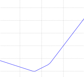
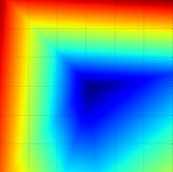
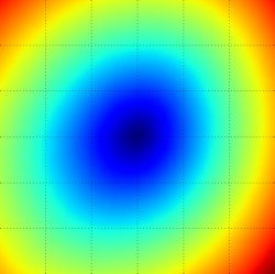
Loss function landscape for the Multiclass SVM (without regularization) for one single example (left,middle) and for a hundred examples (right) in CIFAR-10. Left: one-dimensional loss by only varying a. Middle, Right: two-dimensional loss slice, Blue = low loss, Red = high loss. Notice the piecewise-linear structure of the loss function. The losses for multiple examples are combined with average, so the bowl shape on the right is the average of many piece-wise linear bowls (such as the one in the middle).
We can explain the piecewise-linear structure of the loss function by examining the math. For a single example we have:
It is clear from the equation that the data loss for each example is a sum of (zero-thresholded due to the \(max(0,−)\) function) linear functions of \(W\). Moreover, each row of \(W\) (i.e. \(w_j\)) sometimes has a positive sign in front of it (when it corresponds to a wrong class for an example), and sometimes a negative sign (when it corresponds to the correct class for that example). To make this more explicit, consider a simple dataset that contains three 1-dimensional points and three classes. The full SVM loss (without regularization) becomes:
Since these examples are 1-dimensional, the data \(x_i\) and weights \(w_j\) are numbers. Looking at, for instance, \(w_0\), some terms above are linear functions of \(w_0\) and each is clamped at zero. We can visualize this as follows:
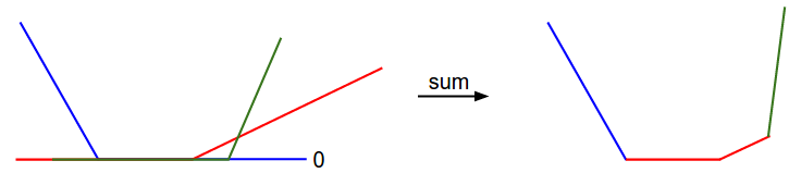
1-dimensional illustration of the data loss. The \(x\)-axis is a single weight and the \(y\)-axis is the loss. The data loss is a sum of multiple terms, each of which is either independent of a particular weight, or a linear function of it that is thresholded at zero. The full SVM data loss is a 30,730-dimensional version of this shape.
As an aside, you may have guessed from its bowl-shaped appearance that the SVM cost function is an example of a convex function [1]. There is a large amount of literature devoted to efficiently minimizing these types of functions, and you can also take a Stanford class on the topic (convex optimization [2]). Once we extend our score functions ff to Neural Networks our objective functions will become non-convex, and the visualizations above will not feature bowls but complex, bumpy terrains.
Non-differentiable loss functions. As a technical note, you can also see that the kinks in the loss function (due to the max operation) technically make the loss function non-differentiable because at these kinks the gradient is not defined. However, the subgradient still exists and is commonly used instead. In this class will use the terms subgradient [3] and gradient interchangeably.
| [1] | https://en.wikipedia.org/wiki/Convex_function |
| [2] | http://stanford.edu/~boyd/cvxbook/ |
| [3] | https://en.wikipedia.org/wiki/Subderivative |